Fake News Vs Real News

Fake News Vs Real News#

In this political landscape “Fake News” is a big buzz word, defining it is a discussion for it self but what we have here is a collections of verifiably falsified reportings paired with reporting on true events. The difference between “fake news” and “real news” is real news isn’t trying to convince you of anything its just the truth being reported on, fake news is actively trying to present skewed facts with the intent to change the readers mind. Through the use of AI tools we can see there is a data driven difference that can be realized to help us determine if something is falsified. While I’d never expect this kind of analysis to change someones mind its at least an unignorable fact that “Fake news” is at least structurally different in its presentation.

from sklearn.feature_extraction import text
from sklearn.metrics.pairwise import euclidean_distances
from sklearn import datasets
import pandas as pd
import numpy as np
import seaborn as sns
from sklearn.naive_bayes import MultinomialNB
from sklearn.model_selection import train_test_split
from sklearn.metrics import confusion_matrix, classification_report
from sklearn.feature_extraction.text import CountVectorizer
from sklearn.model_selection import GridSearchCV
from sklearn.model_selection import cross_val_score

news_df = pd.read_csv('fake_or_real_news.csv')

news_df.head()

	id	title	text	label
0	8476	You Can Smell Hillary’s Fear	Daniel Greenfield, a Shillman Journalism Fello...	FAKE
1	10294	Watch The Exact Moment Paul Ryan Committed Pol...	Google Pinterest Digg Linkedin Reddit Stumbleu...	FAKE
2	3608	Kerry to go to Paris in gesture of sympathy	U.S. Secretary of State John F. Kerry said Mon...	REAL
3	10142	Bernie supporters on Twitter erupt in anger ag...	— Kaydee King (@KaydeeKing) November 9, 2016 T...	FAKE
4	875	The Battle of New York: Why This Primary Matters	It's primary day in New York and front-runners...	REAL

news_df.shape

(6335, 4)

Results for Titles#

Looking at the crossVal scores we see that training and testing scores are fairly close to eachother for both CountVectorizer and TFIDF. CountVectorizer has a lead of 4% in the test cross vals but they are equal in the training data. The closness in training data makes me think this is an overfitting issue and since there is only a 4% difference in test neither is really better than the other.

news_titles_df = news_df.drop(columns=['text'])
news_titles_df.head(1)

	id	title	label
0	8476	You Can Smell Hillary’s Fear	FAKE

news_titles_df.shape

(6335, 3)

Features and Target:

titles_X = news_titles_df['title']
titles_y = news_titles_df['label']

Initial Splits

X_train_titles, X_test_titles, y_train_titles, y_test_titles = train_test_split(titles_X, titles_y, test_size=0.2)

Instantiate, fit, and vectorize. We build and fit X_train_titles_vec than we transform X_test_titles_vec based off the built vocabulary

titles_counts =  CountVectorizer()

X_train_titles_vec = titles_counts.fit_transform(X_train_titles) #Build Vocab

X_test_titles_vec = titles_counts.transform(X_test_titles)

Instantiate and fit classifier

clf_titles = MultinomialNB()
clf_titles.fit(X_train_titles_vec, y_train_titles)

MultinomialNB()

In a Jupyter environment, please rerun this cell to show the HTML representation or trust the notebook.
On GitHub, the HTML representation is unable to render, please try loading this page with nbviewer.org.

Title Scoring

clf_titles.score(X_train_titles_vec, y_train_titles)

0.9398184688239937

clf_titles.score(X_test_titles_vec, y_test_titles)

0.819258089976322

Optimize:#

clf_titles_2 = MultinomialNB()

params = {'alpha': np.linspace(0.01, 1, 10)}

clf_titles_op = GridSearchCV(clf_titles_2, params)

clf_titles_op.fit(X_train_titles_vec, y_train_titles)

GridSearchCV(estimator=MultinomialNB(),
         param_grid={&#x27;alpha&#x27;: array([0.01, 0.12, 0.23, 0.34, 0.45, 0.56, 0.67, 0.78, 0.89, 1.  ])})</pre><b>In a Jupyter environment, please rerun this cell to show the HTML representation or trust the notebook. <br />On GitHub, the HTML representation is unable to render, please try loading this page with nbviewer.org.</b></div><div class="sk-container" hidden><div class="sk-item sk-dashed-wrapped"><div class="sk-label-container"><div class="sk-label fitted sk-toggleable"><input class="sk-toggleable__control sk-hidden--visually" id="sk-estimator-id-2" type="checkbox" ><label for="sk-estimator-id-2" class="sk-toggleable__label fitted sk-toggleable__label-arrow fitted">&nbsp;&nbsp;GridSearchCV<a class="sk-estimator-doc-link fitted" rel="noreferrer" target="_blank" href="https://scikit-learn.org/1.4/modules/generated/sklearn.model_selection.GridSearchCV.html">?<span>Documentation for GridSearchCV</span></a><span class="sk-estimator-doc-link fitted">i<span>Fitted</span></span></label><div class="sk-toggleable__content fitted"><pre>GridSearchCV(estimator=MultinomialNB(),
         param_grid={&#x27;alpha&#x27;: array([0.01, 0.12, 0.23, 0.34, 0.45, 0.56, 0.67, 0.78, 0.89, 1.  ])})</pre></div> </div></div><div class="sk-parallel"><div class="sk-parallel-item"><div class="sk-item"><div class="sk-label-container"><div class="sk-label fitted sk-toggleable"><input class="sk-toggleable__control sk-hidden--visually" id="sk-estimator-id-3" type="checkbox" ><label for="sk-estimator-id-3" class="sk-toggleable__label fitted sk-toggleable__label-arrow fitted">estimator: MultinomialNB</label><div class="sk-toggleable__content fitted"><pre>MultinomialNB()</pre></div> </div></div><div class="sk-serial"><div class="sk-item"><div class="sk-estimator fitted sk-toggleable"><input class="sk-toggleable__control sk-hidden--visually" id="sk-estimator-id-4" type="checkbox" ><label for="sk-estimator-id-4" class="sk-toggleable__label fitted sk-toggleable__label-arrow fitted">&nbsp;MultinomialNB<a class="sk-estimator-doc-link fitted" rel="noreferrer" target="_blank" href="https://scikit-learn.org/1.4/modules/generated/sklearn.naive_bayes.MultinomialNB.html">?<span>Documentation for MultinomialNB</span></a></label><div class="sk-toggleable__content fitted"><pre>MultinomialNB()</pre></div> </div></div></div></div></div></div></div></div></div>


clf_titles_op.best_params_


{'alpha': 0.89}


Training Scores:
clf_titles_op.score(X_train_titles_vec, y_train_titles)


0.941397000789266


cross_val_score(clf_titles_op, X_train_titles_vec, y_train_titles)


array([0.80769231, 0.81065089, 0.79980276, 0.8213228 , 0.80454097])


np.mean(cross_val_score(clf_titles_op, X_train_titles_vec, y_train_titles))


0.8088019455169582


Testing Score:
clf_titles_op.score(X_test_titles_vec, y_test_titles)


0.8200473559589582


cross_val_score(clf_titles_op, X_test_titles_vec, y_test_titles)


array([0.7992126 , 0.7480315 , 0.7826087 , 0.75494071, 0.78656126])


np.mean(cross_val_score(clf_titles_op, X_test_titles_vec, y_test_titles))


0.7742709532849895

TF-IDF for Titles#

titles_tfidf = text.TfidfTransformer()

X_train_titles_tfidf = titles_tfidf.fit_transform(X_train_titles_vec) 

X_test_titles_tfidf = titles_tfidf.transform(X_test_titles_vec)

clf_tfidf_titles = MultinomialNB(alpha=0.67)

Use Prevoius Optimization

clf_tfidf_titles.fit(X_train_titles_tfidf, y_train_titles)

MultinomialNB(alpha=0.67)

In a Jupyter environment, please rerun this cell to show the HTML representation or trust the notebook.
On GitHub, the HTML representation is unable to render, please try loading this page with nbviewer.org.

Training Score:

clf_tfidf_titles.score(X_train_titles_tfidf, y_train_titles)

0.9485003946329913

cross_val_score(clf_tfidf_titles, X_train_titles_tfidf, y_train_titles)

array([0.80571992, 0.80276134, 0.79191321, 0.82230997, 0.80256663])

np.mean(cross_val_score(clf_tfidf_titles, X_train_titles_tfidf, y_train_titles))

0.8050542162927311

Testing Score

clf_tfidf_titles.score(X_test_titles_tfidf, y_test_titles)

0.8153117600631413

cross_val_score(clf_tfidf_titles, X_test_titles_tfidf, y_test_titles)

array([0.78346457, 0.7519685 , 0.76284585, 0.7826087 , 0.75889328])

np.mean(cross_val_score(clf_tfidf_titles, X_test_titles_tfidf, y_test_titles))

0.7679561793906197

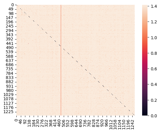
fake_i = np.where(y_test_titles == 'FAKE')[0]
true_i = np.where(y_test_titles == 'REAL')[0]

subset_rows = np.concatenate([fake_i,true_i])
subset_rows

array([   0,    2,    4, ..., 1263, 1264, 1265], dtype=int64)

sns.heatmap(euclidean_distances(X_test_titles_tfidf[subset_rows]))

<Axes: >

png

Results for text#

We see much higher scores than titles with about a 10% increase in testing and trainig crossVal scores. Something interesting is optimizing MultinomialNB() did actually show better results with a lower Alpha. The training data for both countVec and TFIDF are again almost Identical, this is again mostlikely due to overfitting.

news_text_df = news_df.drop(columns=['title'])

text_X = news_text_df['text']
text_y = news_text_df['label']
# Get splits for text

X_train_text, X_test_text, y_train_text, y_test_text = train_test_split(text_X, text_y)

news_text_df.shape

(6335, 3)

Instantiate and fit classifier

text_counts =  CountVectorizer()
X_train_text_vec = text_counts.fit_transform(X_train_text) #Build Vocab
X_test_text_vec = text_counts.transform(X_test_text)

clf_text = MultinomialNB()
clf_text.fit(X_train_text_vec, y_train_text)

MultinomialNB()

In a Jupyter environment, please rerun this cell to show the HTML representation or trust the notebook.
On GitHub, the HTML representation is unable to render, please try loading this page with nbviewer.org.

clf_text.score(X_train_text_vec, y_train_text)

0.940223110924016

clf_text.score(X_test_text_vec, y_test_text)

0.8907828282828283

Optimize:#

clf_text_2 = MultinomialNB()
params_text = {'alpha': np.linspace(0.01, 1, 10)}
clf_text_op = GridSearchCV(clf_text_2, params_text)
clf_text_op.fit(X_train_text_vec, y_train_text)

GridSearchCV(estimator=MultinomialNB(),
         param_grid={&#x27;alpha&#x27;: array([0.01, 0.12, 0.23, 0.34, 0.45, 0.56, 0.67, 0.78, 0.89, 1.  ])})</pre><b>In a Jupyter environment, please rerun this cell to show the HTML representation or trust the notebook. <br />On GitHub, the HTML representation is unable to render, please try loading this page with nbviewer.org.</b></div><div class="sk-container" hidden><div class="sk-item sk-dashed-wrapped"><div class="sk-label-container"><div class="sk-label fitted sk-toggleable"><input class="sk-toggleable__control sk-hidden--visually" id="sk-estimator-id-7" type="checkbox" ><label for="sk-estimator-id-7" class="sk-toggleable__label fitted sk-toggleable__label-arrow fitted">&nbsp;&nbsp;GridSearchCV<a class="sk-estimator-doc-link fitted" rel="noreferrer" target="_blank" href="https://scikit-learn.org/1.4/modules/generated/sklearn.model_selection.GridSearchCV.html">?<span>Documentation for GridSearchCV</span></a><span class="sk-estimator-doc-link fitted">i<span>Fitted</span></span></label><div class="sk-toggleable__content fitted"><pre>GridSearchCV(estimator=MultinomialNB(),
         param_grid={&#x27;alpha&#x27;: array([0.01, 0.12, 0.23, 0.34, 0.45, 0.56, 0.67, 0.78, 0.89, 1.  ])})</pre></div> </div></div><div class="sk-parallel"><div class="sk-parallel-item"><div class="sk-item"><div class="sk-label-container"><div class="sk-label fitted sk-toggleable"><input class="sk-toggleable__control sk-hidden--visually" id="sk-estimator-id-8" type="checkbox" ><label for="sk-estimator-id-8" class="sk-toggleable__label fitted sk-toggleable__label-arrow fitted">estimator: MultinomialNB</label><div class="sk-toggleable__content fitted"><pre>MultinomialNB()</pre></div> </div></div><div class="sk-serial"><div class="sk-item"><div class="sk-estimator fitted sk-toggleable"><input class="sk-toggleable__control sk-hidden--visually" id="sk-estimator-id-9" type="checkbox" ><label for="sk-estimator-id-9" class="sk-toggleable__label fitted sk-toggleable__label-arrow fitted">&nbsp;MultinomialNB<a class="sk-estimator-doc-link fitted" rel="noreferrer" target="_blank" href="https://scikit-learn.org/1.4/modules/generated/sklearn.naive_bayes.MultinomialNB.html">?<span>Documentation for MultinomialNB</span></a></label><div class="sk-toggleable__content fitted"><pre>MultinomialNB()</pre></div> </div></div></div></div></div></div></div></div></div>


clf_text_op.best_params_


{'alpha': 0.01}


Train scores:
clf_text_op.score(X_train_text_vec, y_train_text)


0.9722163754998948


cross_val_score(clf_text_op, X_train_text_vec, y_train_text)


array([0.88643533, 0.90631579, 0.90105263, 0.89894737, 0.89894737])


np.mean(cross_val_score(clf_text_op, X_train_text_vec, y_train_text))


0.8983396978250042


Test Scores:
clf_text_op.score(X_test_text_vec, y_test_text)


0.9034090909090909


cross_val_score(clf_text_op, X_test_text_vec, y_test_text)


array([0.86750789, 0.84542587, 0.86119874, 0.87066246, 0.88924051])


np.mean(cross_val_score(clf_text_op, X_test_text_vec, y_test_text))


0.8668070918021004

TF-IDF for Body Text#

text_tfidf = text.TfidfTransformer()
X_train_text_tfidf = text_tfidf.fit_transform(X_train_text_vec) 
X_test_text_tfidf = text_tfidf.transform(X_test_text_vec)
clf_tfidf_text = MultinomialNB(alpha=0.1) #Used previous optimization
clf_tfidf_text.fit(X_train_text_tfidf, y_train_text)

MultinomialNB(alpha=0.1)

In a Jupyter environment, please rerun this cell to show the HTML representation or trust the notebook.
On GitHub, the HTML representation is unable to render, please try loading this page with nbviewer.org.

Training scores

clf_tfidf_text.score(X_train_text_tfidf, y_train_text)

0.9667438434013892

cross_val_score(clf_tfidf_text, X_train_text_tfidf, y_train_text)

array([0.89064143, 0.91473684, 0.89789474, 0.88842105, 0.89473684])

np.mean(cross_val_score(clf_tfidf_text, X_train_text_tfidf, y_train_text))

0.8972861807515635

Test Scores:

clf_tfidf_text.score(X_test_text_tfidf, y_test_text)

0.9097222222222222

cross_val_score(clf_tfidf_text, X_test_text_tfidf, y_test_text)

array([0.85488959, 0.86435331, 0.88012618, 0.83280757, 0.87025316])

np.mean(cross_val_score(clf_tfidf_text, X_test_text_tfidf, y_test_text))

0.8604859641416762

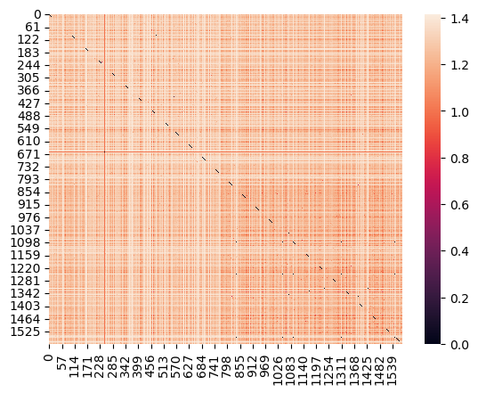
fake_i_text = np.where(y_test_text == 'FAKE')[0]
true_i_text = np.where(y_test_text == 'REAL')[0]
subset_rows = np.concatenate([fake_i_text, true_i_text])
sns.heatmap(euclidean_distances(X_test_text_tfidf[subset_rows]))

<Axes: >

png

Summary#

Using the whole body text of articles is more telling of weather its fake or not. Its clear that feeding the models with more data showed better results, body text having a higher word count allowed for more comparison and complex matrices. The trends in this data show MultinomialNB will start to plateau with these kinds of predictions. Titles can have maybe 10 unique words at most where the articles have much much more, a quick google search shows on average a single paragraph has about 200 words. This shows that feeding MultinomialNB even more articles/titles will have diminishing returns, this points to the need of a more complex model.

Fake News Vs Real News

Contents

Fake News Vs Real News#

Results for Titles#

Optimize:#

TF-IDF for Titles#

Results for text#

Optimize:#

TF-IDF for Body Text#

Summary#